Week 2 - Exponential population growth

In part 1, we will solve the differential equation for exponential population growth and visualize how the population sizes change over time.

Part 1 - Numerical solution using the package deSolve

Two main phases:

Model specification: specify the structure of differential equation model
Model application: set the time steps, initial population size and model parameters (e.g., intrinsic population growth rate \(r\)), and then solve the equation model

Consider the model \[ \frac{dN}{dt} = rN \] where \(N\) is population size and \(r\) is the intrinsic growth rate.

###### part 1 ######
# install.packages("deSolve")
library(deSolve)

### (1) Model specification
exponential_model <- function(times, state, parms) {
  with(as.list(c(state, parms)), {
    dN_dt = r*N  # Exponential growth equation
    return(list(c(dN_dt)))  # Return the results
  })
}

Set the time steps, initial population size and model parameters.

### (2) Model application
times <- seq(0, 10, by = 0.1)  # Time steps to integrate over
state <- c(N = 10)  # Initial population size
parms <- c(r = 1.5)  # Intrinsic growth rate

Solve the equation by ode() numerically.

# Run the ode solver
pop_size <- ode(func = exponential_model, times = times, y = state, parms = parms)

# Take a look at the results
head(pop_size)

##      time        N
## [1,]  0.0 10.00000
## [2,]  0.1 11.61834
## [3,]  0.2 13.49860
## [4,]  0.3 15.68313
## [5,]  0.4 18.22120
## [6,]  0.5 21.17002

Visualization

plot(N ~ time, data = pop_size)

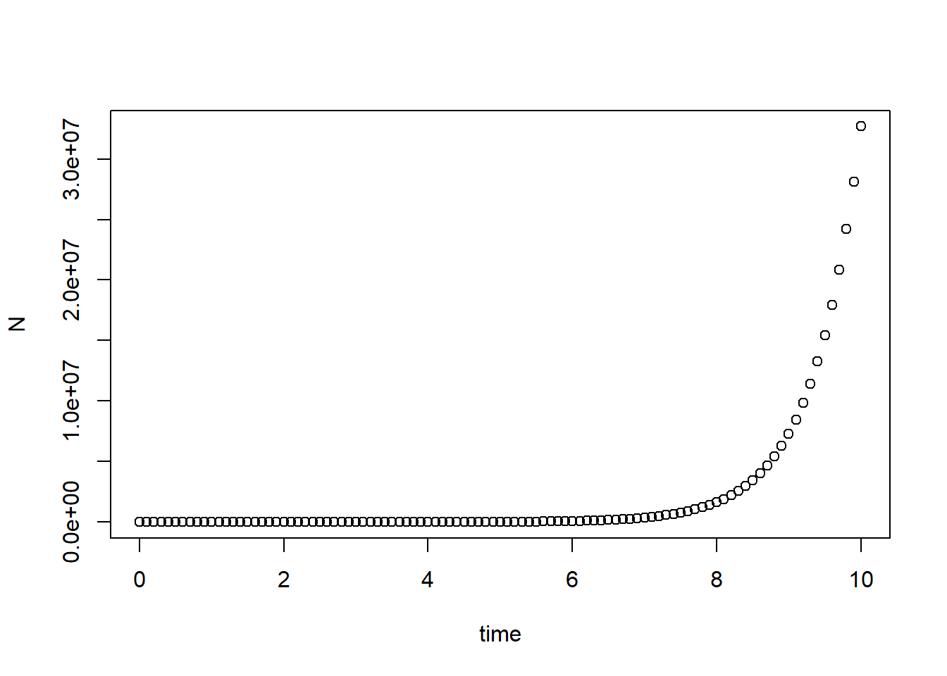
Compare simulation result with analytic solution, which is \[ N(t) = N_0\exp\{rt\} \]

par(mfrow = c(1,2))
plot(N ~ time, data = pop_size) # Plot simulation data
curve(state[1]*exp(parms[1]*x), col = "red", add = T) # Adding analytic solution
plot(N ~ time, data = pop_size, log = "y") # Plot logged simulation data
curve(state[1]*exp(parms[1]*x), col = "red", add = T) # Adding analytic solution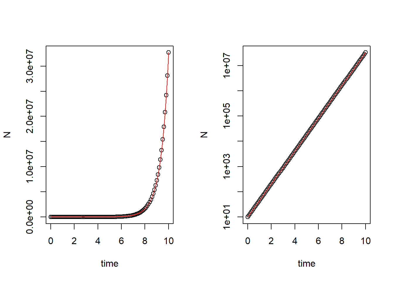

Part 2 - Comparing different ode solvers and different time intervals
In default of ode(), the equations are solved by LSODA method. We can change the method by modifying the argument method in ode().

###### part 2 ######
# Original setting
times <- seq(0, 10, by = 0.1)  # Time steps to integrate over
state <- c(N = 10)  # Initial population size
parms <- c(r = 1.5)  # Intrinsic growth rate
# Default: LSODA
pop_size <- ode(func = exponential_model, times = times, y = state, parms = parms)

# Euler's method
pop_size_1 <- ode(func = exponential_model, times = times, y = state, parms = parms, method = "euler")

# Compare different method
par(mfrow = c(1,2))
plot(N ~ time, data = pop_size, main = "LSODA")
curve(state[1]*exp(parms[1]*x), times[1], times[length(times)], col = "red", add = T) # correct curve
plot(N ~ time, data = pop_size_1, main = "Euler")
curve(state[1]*exp(parms[1]*x), times[1], times[length(times)], col = "red", add = T) # correct curve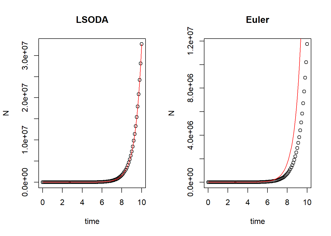

# Different time intervals
times_1 <- seq(0, 10, by = 1)  # time steps to integrate over
times_2 <- seq(0, 10, by = 0.1)  # time steps to integrate over
times_3 <- seq(0, 10, by = 0.01)  # time steps to integrate over

# Euler's method
pop_size_1 <- ode(func = exponential_model, times = times_1, y = state, parms = parms, method = "euler")
pop_size_2 <- ode(func = exponential_model, times = times_2, y = state, parms = parms, method = "euler")
pop_size_3 <- ode(func = exponential_model, times = times_3, y = state, parms = parms, method = "euler")

# Compare different time intervals
par(mfrow = c(1,3))
plot(N ~ time, data = pop_size_1, main = "Time intervals = 1")
curve(state[1]*exp(parms[1]*x), col = "red", add = T) # correct curve
plot(N ~ time, data = pop_size_2, main = "Time intervals = 0.1")
curve(state[1]*exp(parms[1]*x), col = "red", add = T) # correct curve
plot(N ~ time, data = pop_size_3, main = "Time intervals = 0.01")
curve(state[1]*exp(parms[1]*x), col = "red", add = T) # correct curve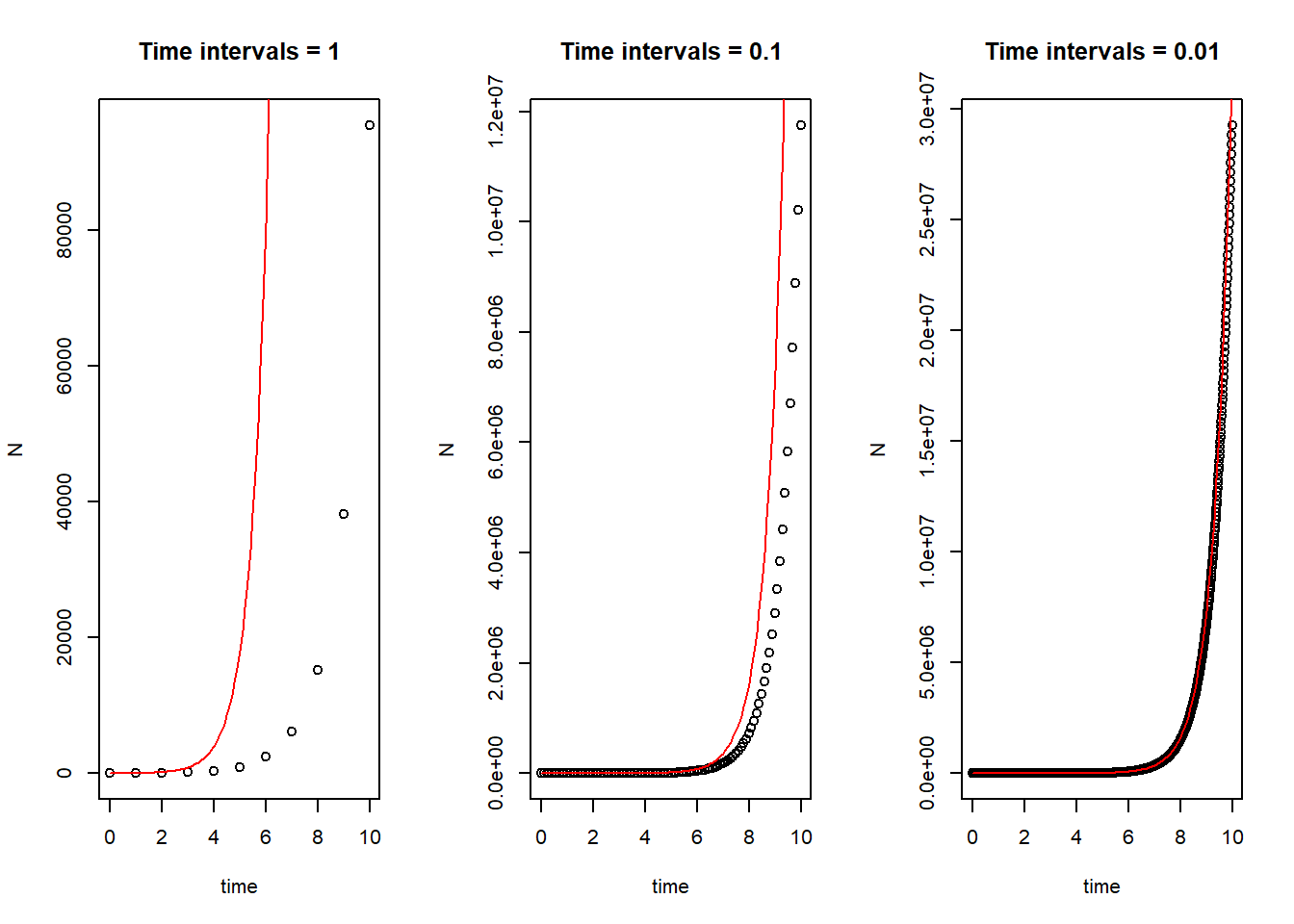

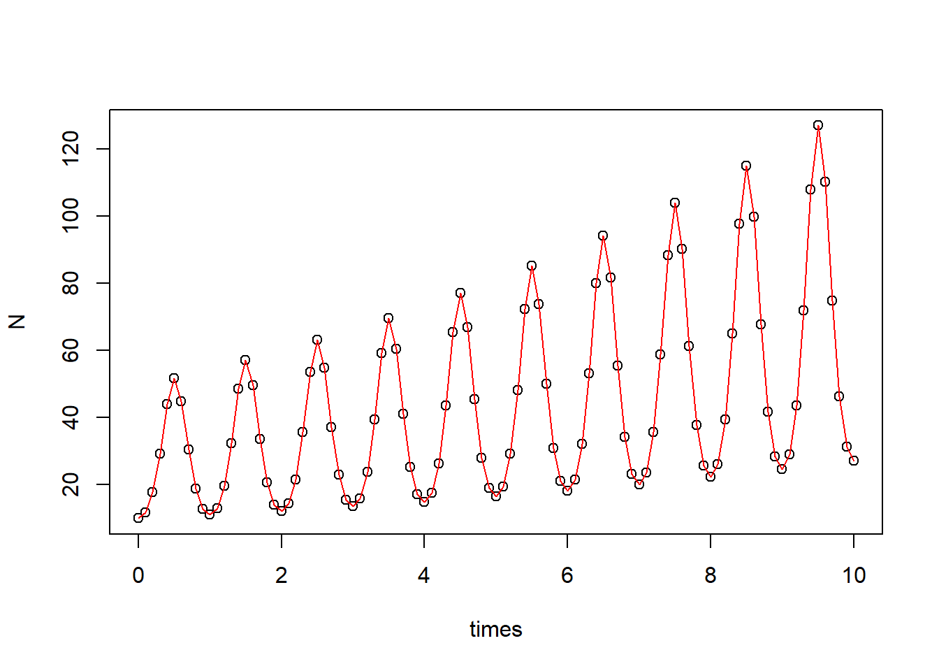
Part 3 - Solving exponential growth model with fluctuating growth rate
Consider the model \[ \frac{dN}{dt} = r(t)N \ \text{, } r(t) = \overline{r} + \sigma\sin(\omega t) \] where \(\overline{r}\) and \(\omega\) are constants. The analytic solution of the ode model is \[ N(t) = N_0\exp\{\overline{r}t - \frac{\sigma}{\omega}[\cos(\omega t) - 1]\} \]

###### part 3 ######
### Model specification
exponential_model_fluc <- function(times, state, parms) {
  with(as.list(c(state, parms)), {
    dN_dt = (r_bar + sigma*sin(omega*times))*N  # exponential growth equation
    return(list(c(dN_dt)))  # return the results
  })
}

### Parameters
times <- seq(0, 10, by = 0.1)  # time steps to integrate over
state <- c(N = 10)  # initial population size
parms <- c(r_bar = 1.5, sigma = 5, omega = 2*pi)  # intrinsic growth rate

Plot \(r(t)\)

### Fluctuating growth rate
r = parms[1] + parms[2]*sin(parms[3]*times)
plot(r ~ times, type = "l")

### Solving model
pop_size <- ode(func = exponential_model_fluc, times = times, y = state, parms = parms)

### Plotting
plot(N ~ times, data = pop_size)
curve(state[1]*exp(parms[1]*x - parms[2]/parms[3]*(cos(parms[3]*x) - 1)), add = T, col = "red") # correct curve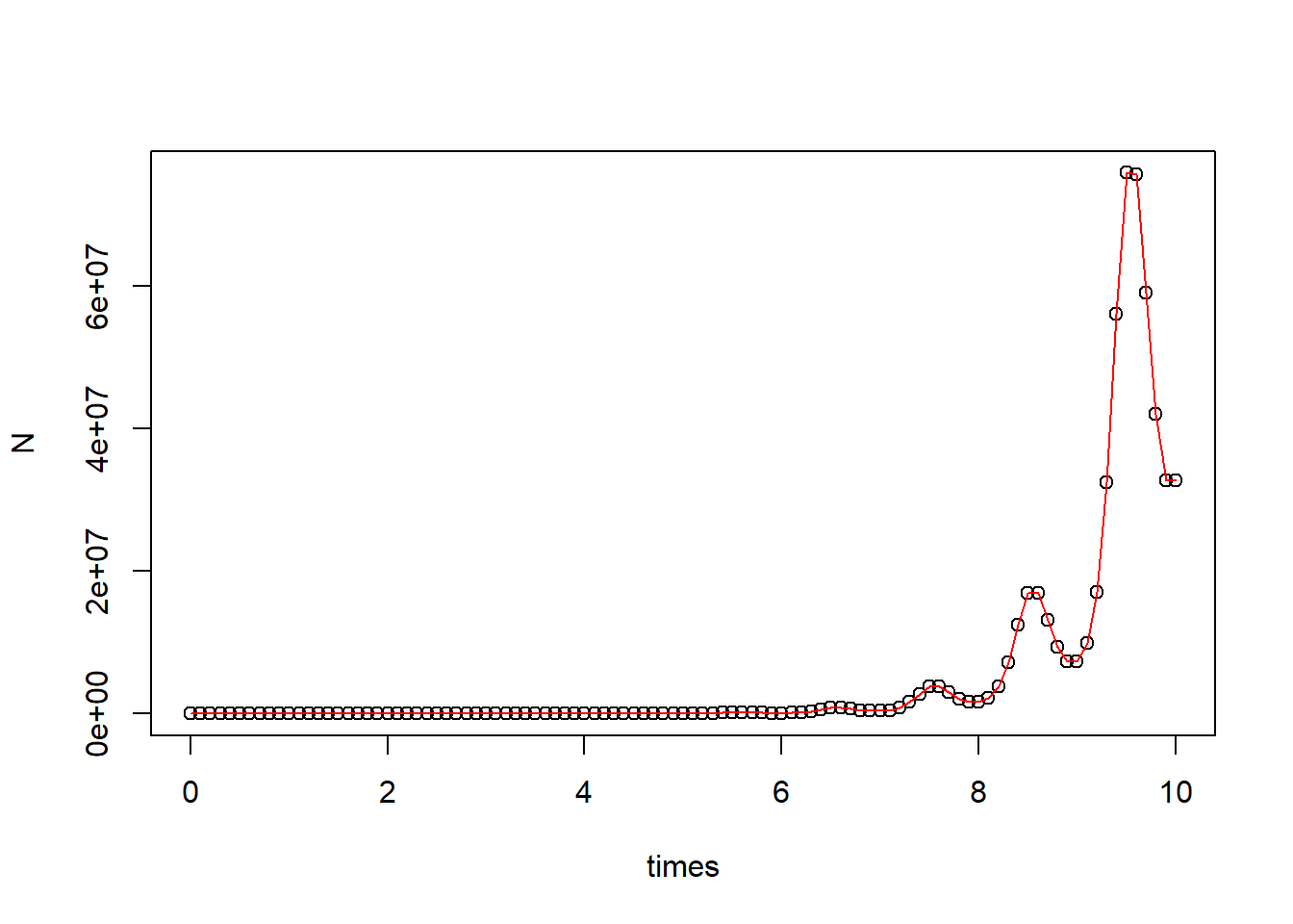

plot(N ~ times, data = pop_size, log = "y")
curve(state[1]*exp(parms[1]*x - parms[2]/parms[3]*(cos(parms[3]*x) - 1)), add = T, col = "red") # correct curve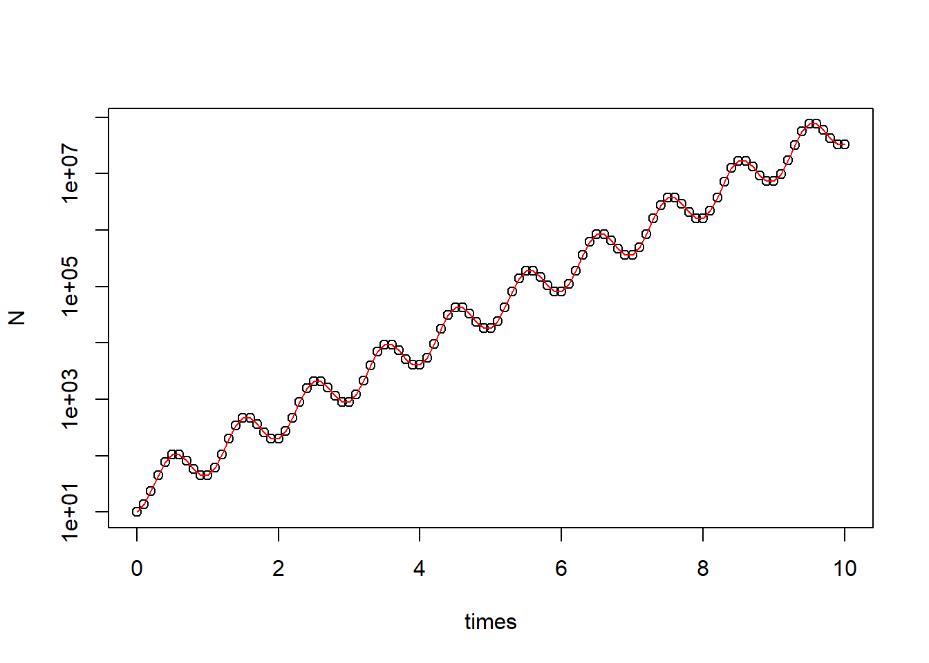

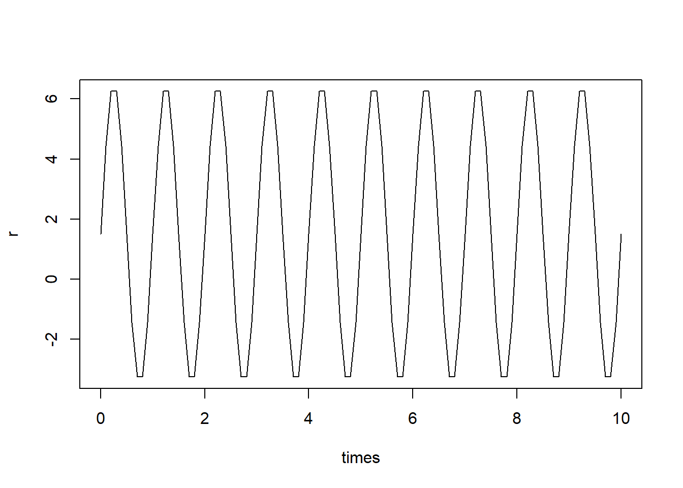
Adjust \(\overline{r}\)

### Parameters
times <- seq(0, 10, by = 0.1)  # time steps to integrate over
state <- c(N = 10)  # initial population size
parms <- c(r_bar = 0.1, sigma = 5, omega = 2*pi)  # intrinsic growth rate

### Fluctuating growth rate
r = parms[1] + parms[2]*sin(parms[3]*times)
plot(r ~ times, type = "l")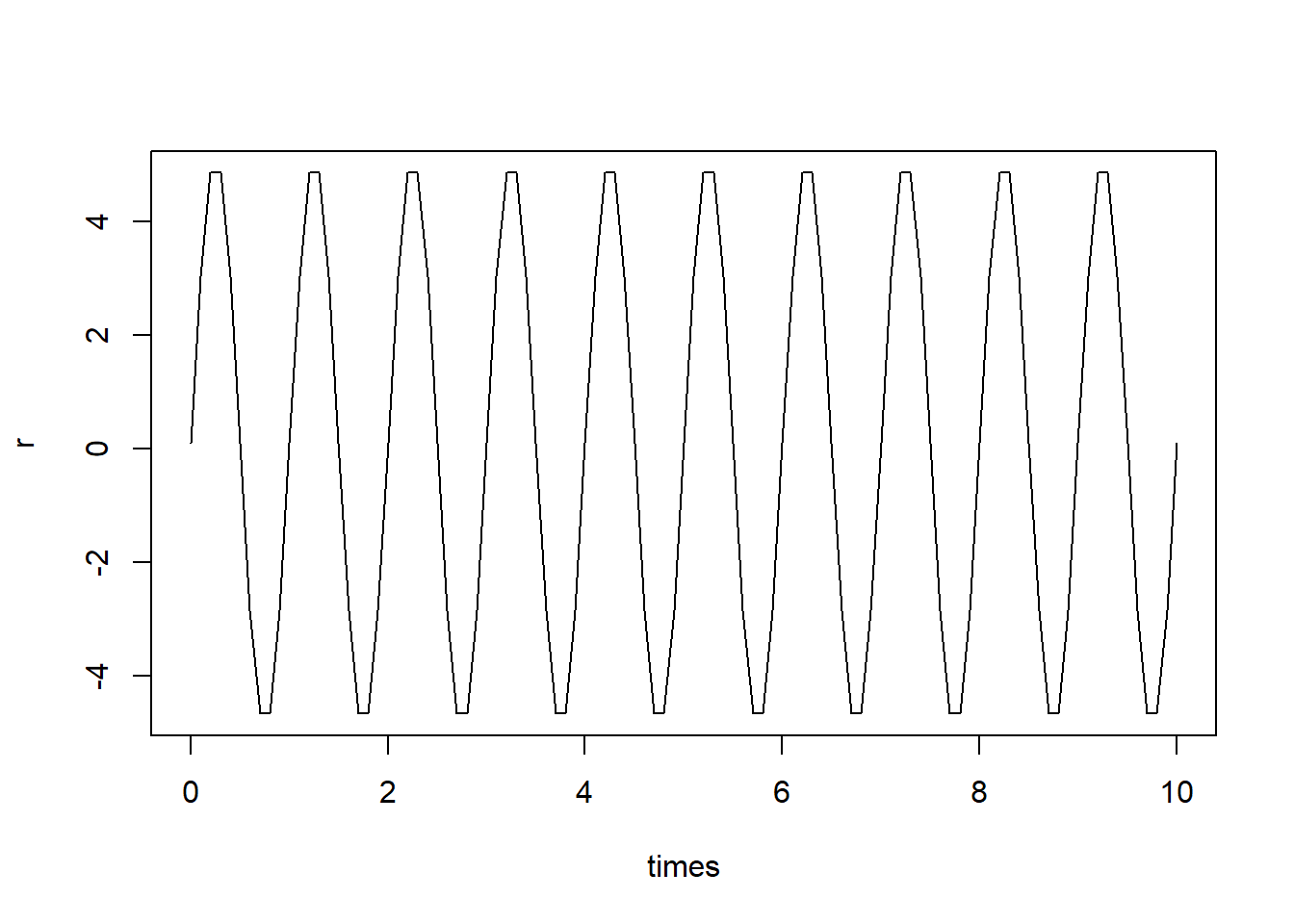

### Solving model
pop_size <- ode(func = exponential_model_fluc, times = times, y = state, parms = parms)

### Plotting
plot(N ~ times, data = pop_size)
curve(state[1]*exp(parms[1]*x - parms[2]/parms[3]*(cos(parms[3]*x) - 1)), add = T, col = "red") # correct curve