Week 4 - Discrete exponential and logistic models

Part 1 - Model the discrete logistic population growth using for loops Model: \[ N_{t+1} = N_t(1+r(1-\frac{N_t}{K})) \]

### (1) Define the discrete logistic growth equation
log_fun <- function(r, N, K){N + r*N*(1-N/K)}

You may modify \(r\) to see the change in stability of equilibrium \(K\).

### (2) Set the parameters
r <- 1.8
K <- 200
N0 <- 10
time <- 100
Parms <- c(r = r, K = K)

### (3) Use for loop to iterate over the time sequence
pop_size <- data.frame(times = 1:time)
pop_size$N[1] <- N0
for(i in 2:time){
  pop_size$N[i] <- log_fun(r = r, N = pop_size$N[i - 1], K = K)
}

### (4) Population trajectory
plot(N ~ times, data = pop_size, type = "l")
abline(h = K, col = "red")
points(N ~ times, data = pop_size)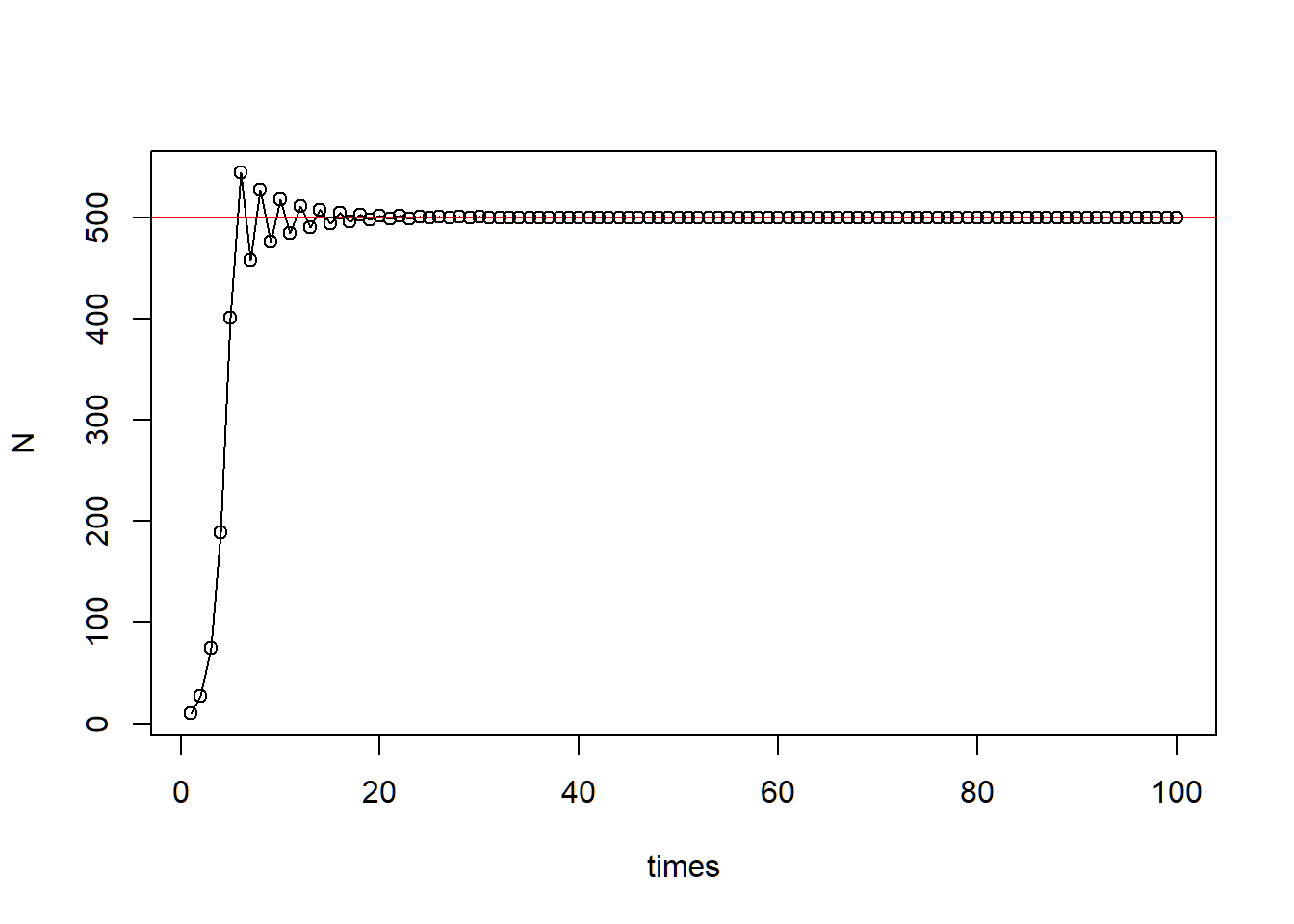

Part 2 - Generic cobweb

###### Part 2: Generic cobweb
### (1) define function
ReturnMap <- function(Func, x0, times, xmax, curve_n = 1000, parms){
  
  # get time series iteration
  x <- rep(x0, times)
  for(i in 2:times){
    x[i] <- Func(x[i-1], parms)
  }
  
  # get fine grid for function curve
  x.grid <- seq(0, xmax, length.out = curve_n)
  y.grid <- Func(x.grid, parms)
  ymax <- max(y.grid, xmax)
  
  # create canvas
  plot(NA, xlim = c(0, xmax), ylim = c(0, ymax), xaxs = "i", yaxs = "i", bty = "l", 
       xlab = expression(N[t]), ylab = expression(N[t+1]))
  abline(a = 0, b = 1, lty = 2, col = "grey50")          
  lines(x.grid, y.grid, col = "steelblue", lwd = 2)      
  
  # cobweb (horizontal to diagonal, vertical up to function)
  segments(x0 = x[1], y0 = 0,   x1 = x[1],   y1 = x[2], col = "firebrick")
  for(i in 2:(times-1)){
    segments(x0 = x[i-1], y0 = x[i],   
             x1 = x[i],   y1 = x[i], col = "firebrick")
    segments(x0 = x[i],   y0 = x[i], 
             x1 = x[i],   y1 = x[i+1], col = "firebrick")
  }
  
}

### (2) Set up discrete logistic function with outside parameters
Logistic <- function(N, parms){
  with(as.list(parms), {
    return(N + r*N*(1-N/K))
  })
}
Parms <- c(r = r, K = K)

### (3) Use the ReturnMap function
ReturnMap(Func = Logistic,
          x0 = 10, 
          times = 150,
          xmax = 310,
          curve_n = 1000, 
          parms = Parms)

Here is a shiny app for the discrete logistic growth model.

Credit to Gen-Chang Hsu

Part 3 - Bifurcation

##### Part 3: Logistic map and bifurcation
### (1) Define the function
RickerPlot <- function(Func, variable, var_vec, x0, times, x_print = 200, parms){
  
  # prepare saving space 
  data_plot <- data.frame(var = rep(var_vec, each = x_print), x = 0)
  
  # change bifurcation parameter
  for (k in 1:length(var_vec)){
    parms[variable] <- var_vec[k]
    x <- rep(x0, times)
    
    # get time series with new bifurcation parameter
    for(i in 2:times){
      x[i] <- Func(x[i-1], parms)
    }
    
    # save the data
    data_plot$x[(1 + (k - 1)*x_print):(k*x_print)] <- x[(times - x_print + 1):times]
  }
  
  # plot 
  plot(x ~ var, data = data_plot, cex = 0.05, pch = 20, 
       xlab = variable, ylab = "Population size")
  
}

#### Discrete logistic function with outside parameters
Logistic <- function(N, parms){
  with(as.list(parms), {
    return(N + r*N*(1-N/K))
  })
}

### (2) Parameter setting
Parms <- c(r = r, K = K)
r_seq <- seq(from = 1.8, to = 3, by = 0.001)

### (3) Use generic ricker plot function
RickerPlot(Func = Logistic, 
           variable = "r", 
           var_vec = r_seq, 
           x0 = 10, 
           times = 500, 
           x_print = 100, 
           parms = Parms)